

Part 2 - What impact do surface shadows have on a point cloud generated using photogrammetry?
- Kenny McLean
- Dec 26, 2016
- 7 min read
This brief is continuation of the high level overview of the potential problem posed by shadows present when creating an elevation model using photogrammetry. Since photogrammetry is based on still images, it can only derive data from what is ‘seen’ by the camera. If high contrast areas exist because of meteorological lighting conditions, can these areas impact our resulting point cloud 3D model? Will this variance introduce error into the elevation model? This is the second paper on this topic. It is recommended that you read the first primer in this series as will provide some foundations that are built upon.
This high level overview of the topic is provided solely as introductory guidance for our pilots, planners and post processors.
Methods A suitable target area was chosen that has a uniform surface and contains the requisite shadow. For this we used a groomed pasture that contains shadows from a tree line.
For this brief an eBee RTK was used and the imaging payload was Canon S110. Flight over subject area was conducted at 1300 hours (GMT -5), which provided high solar irradiance of our surface target and sharp contrast on the landscape. Meteorological conditions provided clear sky and low wind (<8 knots).
All data processed in the WGS 84 datum as it will be satisfactory for our purpose. The mission altitude was flown to achieve ground resolution of 5cm / pixel. Mission overlap was set to 70% lat / 80% long and the target area flown with perpendicular legs.
Initial processing was conducted using Pix4D. Settings that deviate from standard 3D Map template are: Image Scale was set to 1 Original Size, No default classification of data points.
Orthomosaic Pictured below (Image 1) is the ortho derived from the mission. This is provided to assist in orienting our readers to the relationship of target areas. These areas were chosen as the ground elevation is relatively flat in each area. Also, these areas were chosen as the shadows contained in each represent a typical cross section of what is normally found in these situations, containing both dark and light shadow effects.
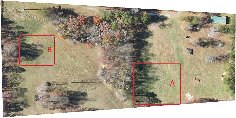
Image 1-Ortho view of subject property.
Analysis of Section B Lets start the conversation in Section B as it is smaller and contains a single point of interest. As we did in the earlier published Part 1, analysis of the area in the shadow and the area beside the shadow will reveal any differential in the cohesion of point cloud data of the surface. We will examine the shadow region by using: 1) A cross section of point cloud using a mensuration line through the shadow region. 2) Colorize the point cloud showing deviation 0.1m +/- from the Median Z . Image 2 at right is a RGB view of Section B and shows the tree shadow across the field surface. Our mensuration line is shown (dotted) with cross sections spaced at 5 Meter intervals.

Image 2 - Section B Mensuration line (dotted) with 5 meter spacing.
Image 3 below shows how noisy the point cloud is within the shadow region. The sample of data points represented below (Image 3) is generated by a cross section view that is sampled from 0.25 meter wide path along the mensuration line. Image 3 clearly illustrates that the samples from the shadowy area contain less coherent point data. There seems to be serious deviation at the 6-7 meter mark and again 19-24 meter mark. Referring to our RGB view in Image 2, these regions of high divergence correlate to the regions with the darkest shadow component.

Image 3 – point cloud cross section sample along mensuration line.
In Image 4 the points in our region are colorized based on Mean Z. A deviation of +/- 0.1 meter from Mean Z is used. A binary colorization scheme is used where Blue color are points that have positive deviation and Red indicates a negative deviation. Gray colored areas represent points that lie between -0.1 meter and +0.1 meter of the Mean Z, and therefor are considered tightly coherent. The shadow of the tree in our sample region Area B has caused large areas to be incorrect in our point cloud that was generated by Pix4D.

Image 4 –Binary color map of Deviation from Mean Z.
We can conduct a more detailed analysis of this area by creating a heat map using the same subset area of the point cloud. In Image 5 below we have a heat map showing the amount of deviation from Mean Z. Each square is 0.25 meters and shows blue to red gradient color based on the number of points that deviate from Mean Z. The more blue the area hue is, the higher cohesion to Mean Z. Conversely, the more red the area hue is, the greater the deviation from Mean Z.
Starting along the mensuration line (dotted) on the left at 0, our point cloud data appear to be strongly blue (coherent). As we move along the line to the right, the region within the 6-7 meter mark and the region within the 19-24 meter marks are very red as they have the highest deviation (lowest cohesion). In Image 3 (cross section of the point cloud above) we can validate this along the length of the mensuration line.

Image 5 – Heat map of Mean Z deviation.
By comparing the RGB layer with the heat map (Image 6), one can clearly see the heat map directly corresponds to the shadow area.

Image 6 – Side by Side of RGB and Z Deviation heat map.
From this we can conclude that shadows cast on our ground surface have caused some degradation in accuracy when creating a 3D model using photogrammetry.
Analysis of Section A Lets apply the same analysis to Section A. The shadows in Section A are cast by the forest edge and are continuous, as opposed to being from a solitary tree as in Section B. Will these continuous shadows moderate the degradation in point cloud accuracy? Or make it worse.
A mensuration line has been placed in Section A with similar cross sections placed at 5 meter intervals. This is to provide the reader a reference when viewing the various exhibits to make it easier to align our various elements.
Image 7 below is the RGB view of our region that includes a mensuration line with cross sections defined every 5 meters. This line was placed as to pass through areas of shadow that show the greatest effect. It passes through areas of dark shadows, lighter shadows and well lit area. The top half of the image is of the well lit grass and the bottom half is of the largely shaded grass. The grass field is well groomed and uniform throughout our sample area at 4 - 6 inches in height.

Image 7 –RGB area map.
In Image 8 below the same methods are applied to this image area as were discussed earlier in analysis of Section B. The points that are blue or red represent point cloud data that is greater than +/- 0.1 meter relative to Mean Z. And the points that lie between +/- 0.1 meter from Mean Z are gray in color. It is very clear that the grassy areas that are well lit have low deviation and thus is mostly gray. However, the areas of grass that lie in shadow have much higher deviation from Mean Z and have therefor contain high red / blue density distribution.

Image 8 –Binary color map of Deviation from Mean Z.
In Image 9 we apply the same heat map technique, blue to red gradient, that was discussed in the Section B. It is clear that the cohesion of point cloud data diminishes in the grass areas that lie within a shadowy area.

Image 9 –Heat map of Deviation from Mean Z.
Takeaway / Conclusion It is clear that shadows can impact the accuracy of the derived point cloud within the shadow region. Now that we have established there exist less accuracy with shaded areas, the big question is how much error is introduced. From our data sets in this discussion, we can see that the registration of point cloud data in the well lit areas are tight. Certainly for our example, +/- 0.15 meters (+/- 6 inches) proved to be normal in the well lit areas. For most applications this is more than adequate to render an accurate DEM.
But the areas in shadow showed that +/- 1 meter point deviation is common. This can have an undesirable effect on our DEM creation. In Image 10 below we see the impact of the low cohesion of the shadow region from Section B on created DEMs. Using the same cross section of point cloud data as exhibited in Image 3, we add two base lines from sample DEMs. The two solid lines represent elevation derived by using both 1 meter (Dark Blue) and a 2 meter (Aqua) grids to sample the data. The 1 meter grid line show some deviation in the shadow regions, as the weighting of the incorrect points forces an upward or downward trend on the rendered surface. The DEM derived from 2 meter grids is much less subject to these micro trends.

Image 10 – point cloud cross section sample with 1 meter and 2 meter DEM.
Identifying the areas of our target surface that is subject to these shadow induced inaccuracies during post processing can help ensure proper attention is paid to correct.
Since all post processing is based on the accuracy of the point cloud, pilots will need to observe their target area / surfaces and make field accommodations in flight planning to best handle missions with strong shadows that may exist, especially in critical areas.
Other items to be mindful of: 1. the difference in capture time between images containing a shadow as a result of long flight legs as this can make the shadow appear to move when processing. 2. Time of day can be used to address the location of shadows if shadows are located in a critical or desirable area. 3. Adjust camera settings to better handle the high contrast. 4. Conducting missions during high overcast cloud cover can be used to reduce the strength and even presence of shadows.
However, some surfaces or conditions may require LIDAR as the best solution to meet the customer’s needs. Always set customer expectations so that they have an accurate and thorough understanding of what the capabilities are and any limitations that may exist.


Comments